Thermodynamic Integration
Thermodynamic Integration (TI) is a method coming straight from statistical physics. In physics, it is used to compute the difference of free energy between two systems and by creating a path between the two. This might sound sounds very abstract but we are going to go from explaining what it means in physics to a direct application in Bayesian Inference.
The physics approach
Let's first define a simple system, with its state defined by . For example, we could pick a spring (the system), without gravity, friction, etc, and define as the distance from the rest position.
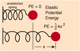 Illustration from http://hydrogen.physik.uni-wuppertal.de/hyperphysics/hyperphysics/hbase/pespr.html
The potential energy of a spring is , where is the spring constant.
Now we could be interested on what is the probability to find the spring in a certain state! This can be done by using the following Gibbs density distribution:
where is the partition function of this system defined as
where is the domain of all the possible states of the system. From a quick glance we can see that the highest probability is when and that this probability decreases when goes away from its rest position. Physics don't like to have any efforts
The free energy is a complex concept which belongs mostly in thermodynamics. It has no real meaning in our example, since thermodynamics is the study of system with many objects. Nonetheless we can still use its definition:
Let's imagine that we have two springs (systems) with different constants and , and associated potential energy function and . We can imagine that we control the variable and create a linear interpolation between the two creating a third intermediate system :
Note that and .
Now the most important result is that we can prove that the difference of free energy is given by:
where is defined by the potential energy . Proof :
What this result tell us is that we can compute the difference of free energy by computing the expectation of the difference of potentials when moving the system from one to another! It is all very nice, but very abstract if you are not a physicist and what does it have to do with Bayesian inference?
Using it in Bayesian Inference
Let's start with the basics: we have , some hypothesis or parameters of a model, and , some observed data! The Bayes theorem states that the posterior is defined as:
where is the likelihood, is the prior, we call the joint distribution and finally is the evidence.
We can rewrite it as an energy model, just as earlier!
where the potential energy is the negative log joint and the partition function is the evidence. We have now the direct connection that the free energy is nothing else than the log evidence.
We have a direct connection between energy models and Bayesian problems! Which leads us to the use of TI for Bayesian inference:
The most difficult part of the Bayes theorem comes from the fact that, except for simple cases, the posterior as well as the evidence are intractable. can be an important quantity to evaluate, if it's not for optimization of the model hyper-parameters, it can be simply for model comparisons. However, computing involves a high-dimensional integral with additional potential issues! That's where Thermodynamic Integration can save the day!
Creating a path from the prior to the posterior
Let's consider two systems again: prior : and the joint distribution . Our intermediate state is given by:
.
The normalized density derived from this potential energy is called a power posterior :
,
which is a posterior for which we reduced the importance of the likelihood.
Performing the thermodynamic integration we derived earlier gives us :
Now let's put this to practice for a very simple use case of a Gaussian prior with a Gaussian likelihood
We take to make a clear difference between and
Of course the posterior can be found analytically but this will help us to evaluate different approaches.
using Plots, Distributions, LaTeXStrings
σ_p = 1.0 # Define your standard deviation for the prior
σ_l = 1.0 # Define your standard deviation for the likelihood
μ_p = 10.0 # define the mean of your prior
prior = Normal(μ_p, σ_p) # prior distribution
likelihood(x) = Normal(x, σ_l) # function returning a distribution given x
y = -10.0
p_prior(x) = pdf(prior, x) # Our prior density function
p_likelihood(x, y) = pdf(likelihood(x), y) # Our likelihood density function
Now we have all the parameters in place we can define the exact posterior and power posterior:
σ_posterior(λ) = sqrt(inv(1/σ_p^2 + λ / σ_l^2))
μ_posterior(y, λ) = σ_posterior(λ) * (λ * y / σ_l^2 + μ_p / σ_p^2)
posterior(y) = Normal(μ_posterior(y, 1.0), σ_posterior(1.0))
p_posterior(x, y) = pdf(posterior(y), x)
power_posterior(y, λ) = Normal(μ_posterior(y, λ), σ_posterior(λ))
p_pow_posterior(x, y, λ) = pdf(power_posterior(y, λ), x)
xgrid = range(-15, 15, length = 400)
plot(xgrid, p_prior , label = "Prior", xlabel = "x")
plot!(xgrid, x->p_likelihood(x, y),label =  "Likelihood")
plot!(xgrid, x->p_posterior(x, y), label = "Posterior") 

We can also visualize the energies themselves
U_A(x) = -logpdf(prior, x)
U_B(x, y) = -logpdf(likelihood(x), y) - logpdf(prior, x)
U_λ(x, y, λ) = -logpdf(prior, x) - λ * logpdf(likelihood(x), y) 
Now we can start evaluating the integrand for multiple . It is standard practice to use an irregular grid with step size
M = 100
λs = ((1:M)./M).^5
expec_λ = zeros(length(λs))
T = 1000
for (i, λ) in enumerate(λs)
    pow_post = power_posterior(y, λ)
    expec_λ[i] = sum(logpdf(likelihood(x), y) for x in rand(pow_post, T)) / T
end 
And we can now compare the sum with the actual value of :
using Trapz, Formatting
logpy = logpdf(posterior(y), y)
s_logpy = fmt(".2f", logpy)
TI_logpy = [trapz(λs[1:i], expec_λ[1:i]) for i in 1:length(λs)] 
Other approaches
Now that's great but how does it compare to other methods? Well we want to compute the integral . The most intuitive way is to sample from the prior to perform a Monte-Carlo integration:
where .
T = 10000
xs = rand(prior, T)
prior_logpy = [log(mean(pdf.(likelihood.(xs[1:i]), y))) for i in 1:T] 
As you can see the result is quite off. The reason is that it happens a lot that the prior and the likelihood have very little overlap. This leads to a huge variance in the estimate of the integral.
Finally there is another approach called the harmonic mean estimator. So far we sampled from power posteriors, the prior but not from the posterior! Most Bayesian inference methods aim at getting samples from the posterior so this would look like an appropriate approach. If we perform naive importance sampling :
this would simply not work. But if we use an unnormalized version of the density we get :
Now replacing by we get the equation :
where . Now the issue with this is that even though both side of the fractions are unbiased, the ratio is not! Experiments tend show this leads to a large bias. Let's have a look for our problem
T = 10000
xs = rand(posterior(y), T)
posterior_logpy = [-log(mean(inv.(pdf.(likelihood.(xs[1:i]), y)))) for i in 1:T] 
As you can see, it's not ideal either. If we now plot all our results together :

We can see that TI gives the most accurate result! For a better estimate, it would be preferable to repeat these estimates multiple times, so I encourage you to try it yourself! Of course other methods exist which I did not cover like Bayesian quadrature and others but this should give you a good idea on what is Thermodynamic Integration.